Tutorial
Model Building
Consider a simple system of chemical reactions given by:
Suppose k0.11 = 1, k0.1 = 1 and there are initially 100 units of A. Then we have the following model string
>>> model_str = """
        const compartment comp1;
        comp1 = 1.0; # volume of compartment

        r1: A => B; k1; # differs from antimony
        r2: B => C; k2; # differs from antimony

        k1 = 0.11;
        k2 = 0.1;
        chem_flag = false;

        A = 100;
        B = 0;
        C = 0;
    """
The format of the model string is based on a subset of the antimony modeling language, but with one key difference. Antimony allows the user to specify custom rate equations for each reaction. cayenne automagically generates the rate equations behind the scenes, and user need only supply the rate constants. The format is discussed below:
Model format
const compartment comp1;
This defines the compartment in which the reactions happen.:
comp1 = 1.0;
This defines the volume of the compartment in which reactions happen. For zero and first order reactions, this number does not matter. For second and third order reactions, varying compartment volume will affect the kinetic outcomes even when the rest of the model is not changed. A blank line after this separates these definitions from the reactions.:
r1: A => B; k1; # differs from antimony
r2: B => C; k2; # differs from antimony
Here r1 and r2 refer to the names of the reactions. This is followed by a colon and the reactants in that reaction. In r1 there is only one reactant, A. Additional reactants or stoichiometries can be written like A + 2B. This is followed by a => which separates reactants and products. Products are written in a fashion similar to the reactants. A semi-colon indicates the end of the products. This is followed by a symbol depicting the rate constant e.g. k1, and the reaction ends with a second semi-colon. A blank line after this separates these reactions from rate-constant assignments.:
k1 = 0.11;
k2 = 0.1;
The rate constants are assigned one per line, with each line ending in a semi-colon. Every rate constant defined in the reactions must be assigned a numerical value at this stage, or cayenne will throw a cayenne.model_io.RateConstantError.:
chem_flag = false;
An additional element that is included at this stage is the chem_flag boolean variable. This is discussed more in detail in the documentation of cayenne.Simulation class under the notes section. Briefly, if
- the system under consideration is a chemical system and the supplied rate constants are in units of molarity or M or mol/L,
chem_flagshould be set totrue - the system under consideration is a biological system and the supplied rate constants are in units of copies/L or CFU/L,
chem_flagshould be set tofalse
A blank line after this separates rate constants from initial values for the species.:
A = 100;
B = 0;
C = 0;
The initial values for species are assigned one per line, with each line ending in a semi-colon. Every species defined in the reactions must be assigned an integer initial value at this stage, or cayenne will throw a cayenne.model_io.InitialStateError.
Warning
Antimony has a set of reserved keywords that cannot be used as species, compartment or variable names, Eg. formula, priority, time, etc. Refer to the antimony documentation for more information.
Note
cayenne only accepts zero, first, second and third order reactions. We decided to not allow custom rate equations for stochastic simulations for two reasons:
- A custom rate equation, such as the Monod equation (see here for background) equation below, may violate the assumptions of stochastic simulations. These assumptions include a well stirred chamber with molecules in Brownian motion, among others.
- An equation resembling the Monod equation, the Michaelis-Menten equation, is grounded chemical kinetic theory. Yet the rate expression (see below) does not fall under 0-3 order reactions supported by
cayenne. However, the elementary reactions that make up the Michaelis-Menten kinetics are first and second order in nature. These elementary reactions can easily be modeled withcayenne, but with the specification of additional constants (see examples). A study shows that using the rate expression of Michaelis-Menten kinetics is valid under some conditions.
Note
The chem_flag is set to True since we are dealing with a chemical system. For defintion of chem_flag, see the notes under the definition of the Simulation class.
These variables are passed to the Simulation class to create an object that represents the current system
>>> from cayenne import Simulation

>>> sim = Simulation.load_model(model_str, "ModelString")
-
class
cayenne.simulation.Simulation(species_names: List[str], rxn_names: List[str], react_stoic: numpy.ndarray, prod_stoic: numpy.ndarray, init_state: numpy.ndarray, k_det: numpy.ndarray, chem_flag: bool = False, volume: float = 1.0)[source]¶ A main class for running simulations.
Parameters: - species_names (List[str]) – List of species names
- rxn_names (List[str]) – List of reaction names
- react_stoic ((ns, nr) ndarray) – A 2D array of the stoichiometric coefficients of the reactants. Reactions are columns and species are rows.
- prod_stoic ((ns, nr) ndarray) – A 2D array of the stoichiometric coefficients of the products. Reactions are columns and species are rows.
- init_state ((ns,) ndarray) – A 1D array representing the initial state of the system.
- k_det ((nr,) ndarray) – A 1D array representing the deterministic rate constants of the system.
- volume (float, optional) – The volume of the reactor vessel which is important for second and higher order reactions. Defaults to 1 arbitrary units.
- chem_flag (bool, optional) – If True, divide by Na (Avogadro’s constant) while calculating
stochastic rate constants. Defaults to
False.
Raises: ValueError– If supplied with order > 3.Examples
>>> V_r = np.array([[1,0],[0,1],[0,0]])
>>> V_p = np.array([[0,0],[1,0],[0,1]])
>>> X0 = np.array([10,0,0])
>>> k = np.array([1,1])
>>> sim = Simulation(V_r, V_p, X0, k)
Notes
Stochastic reaction rates depend on the size of the system for second and third order reactions. By this, we mean the volume of the system in which the reactants are contained. Intuitively, this makes sense considering that collisions between two or more molecules becomes rarer as the size of the system increases. A detailed mathematical treatment of this idea can be found in [3] .
In practice, this means that
volumeandchem_flagneed to be supplied for second and third order reactions.volumerepresents the size of the system containing the reactants.In chemical systems
chem_flagshould generally be set toTrueask_detis specified in units of molarity or M or mol/L. For example, a second order rate constant could be = 0.15 mol / (L s). Then Avogadro’s constant (\(N_a\)) is used for normalization while computingk_stoc(\(c_\mu\) in [3] ) fromk_det.In biological systems,
chem_flagshould be generally be set toFalseask_detis specified in units of copies/L or CFU/L. For example, a second order rate constant could be = 0.15 CFU / (L s).References
[3] (1, 2) Gillespie, D.T., 1976. A general method for numerically simulating the stochastic time evolution of coupled chemical reactions. J. Comput. Phys. 22, 403–434. doi:10.1016/0021-9991(76)90041-3.
Running Simulations
Suppose we want to run 10 repetitions of the system for at most 1000 steps / 40 time units each, we can use the simulate method to do this.
>>> sim.simulate(max_t=40, max_iter=1000, n_rep=10)
-
Simulation.simulate(max_t: float = 10.0, max_iter: int = 1000, seed: int = 0, n_rep: int = 1, n_procs: Optional[int] = 1, algorithm: str = 'direct', debug: bool = False, **kwargs) → None[source]¶ Run the simulation
Parameters: - max_t (float, optional) – The end time of the simulation. The default is 10.0.
- max_iter (int, optional) – The maximum number of iterations of the simulation loop. The default is 1000 iterations.
- seed (int, optional) – The seed used to generate simulation seeds. The default value is 0.
- n_rep (int, optional) – The number of repetitions of the simulation required. The default value is 1.
- n_procs (int, optional) – The number of cpu cores to use for the simulation.
Use
Noneto automatically detect number of cpu cores. The default value is 1. - algorithm (str, optional) – The algorithm to be used to run the simulation.
The default value is
"direct".
Notes
The status indicates the status of the simulation at exit. Each repetition will have a status associated with it, and these are accessible through the
Simulation.results.status_list.- status: int
Indicates the status of the simulation at exit.
1: Succesful completion, terminated when
max_iteriterations reached.2: Succesful completion, terminated when
max_tcrossed.3: Succesful completion, terminated when all species went extinct.
-1: Failure, order greater than 3 detected.
-2: Failure, propensity zero without extinction.
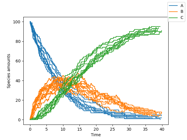
Plotting
To plot the results on the screen, we can simply plot all species concentrations at all the time-points using:
>>> sim.plot()
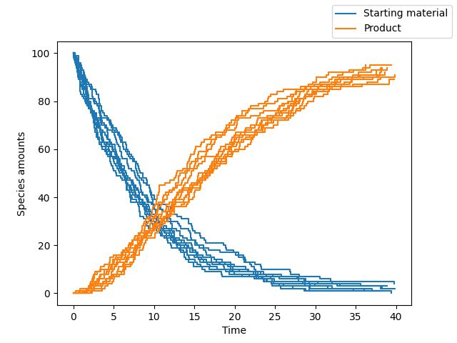
A subset of the species can be plotted along with custom display names by supplying additional arguments to Simulation.plot as follows:
>>> sim.plot(species_names = ["A", "C"], new_names = ["Starting material", "Product"])
By default, calling the plot object returns the matplotlib figure and axis objects. To display the plot, we just do:
>>> sim.plot()
>>> import matplotlib.pyplot as plt
>>> plt.show()
Instead to save the figure directly to a file, we do:
>>> sim.plot()
>>> import matplotlib.pyplot as plt
>>> plt.savefig("plot.png")
-
Simulation.plot(species_names: list = None, new_names: list = None, thinning: int = 1)[source]¶ Plot the simulation
Parameters: - species_names (list, optional) – The names of the species to be plotted (
listofstr). The default isNoneand plots all species. - new_names (list, optional) – The names of the species to be plotted.
The default is
"xi"for speciesi. - thinning (int) – The parameter that controls the sampling Eg. a value of 100 means that 1 point will be sampled every 100 steps The default is 1 (every time-point is sampled)
Returns: - fig (class ‘matplotlib.figure.Figure’) – Figure object of the generated plot.
- ax (class ‘matplotlib.axes._subplots.AxesSubplot) – Axis objected of the generated plot.
- species_names (list, optional) – The names of the species to be plotted (
Note
- The
sim.plotmethod needs to be run after runningsim.simulate - More detailed plots can be created manually by accessing the
sim.resultsobject
Accessing the results
The results of the simulation can be retrieved by accessing the Results object as
   >>> results = sim.results
   >>> results
   <Results species=('A', 'B', 'C') n_rep=10algorithm=direct sim_seeds=[8325804 1484405 2215104 5157699 8222403 7644169 5853461 6739698  374564
2832983]>
The Results object provides abstractions for easy retrieval and iteration over the simulation results. For example you can iterate over every run of the simulation using
>>> for x, t, status in results:
...     pass
You can access the results of the n th run by
>>> nth_result = results[n]
You can also access the final states of all the simulation runs by
>>> final_times, final_states = results.final

# final times of each repetition
>>> final_times
array([6.23502469, 7.67449057, 6.15181435, 8.95810706, 7.12055223,
   7.06535004, 6.07045973, 7.67547689, 9.4218006 , 9.00615099])

# final states of each repetition
>>> final_states
array([[  0,   0, 100],
   [  0,   0, 100],
   [  0,   0, 100],
   [  0,   0, 100],
   [  0,   0, 100],
   [  0,   0, 100],
   [  0,   0, 100],
   [  0,   0, 100],
   [  0,   0, 100],
   [  0,   0, 100]])
You can obtain the state of the system at a particular time using the get_state method. For example to get the state of the system at time t=5.0 for each repetition:
>>> results.get_state(5.0)
[array([ 1,  4, 95]),
array([ 1,  2, 97]),
array([ 0,  2, 98]),
array([ 3,  4, 93]),
array([ 0,  3, 97]),
array([ 0,  2, 98]),
array([ 1,  1, 98]),
array([ 0,  4, 96]),
array([ 1,  6, 93]),
array([ 1,  3, 96])]
Additionally, you can also access a particular species’ trajectory through time across all simulations with the get_species function as follows:
>>> results.get_species(["A", "C"])
This will return a list with a numpy array for each repetition. We use a list here instead of higher dimensional ndarray for the following reason: any two repetitions of a stochastic simulation need not return the same number of time steps.
-
class
cayenne.results.Results(species_names: List[str], rxn_names: List[str], t_list: List[numpy.ndarray], x_list: List[numpy.ndarray], status_list: List[int], algorithm: str, sim_seeds: List[int])[source]¶ A class that stores simulation results and provides methods to access them
Parameters: - species_names (List[str]) – List of species names
- rxn_names (List[str]) – List of reaction names
- t_list (List[float]) – List of time points for each repetition
- x_list (List[np.ndarray]) – List of system states for each repetition
- status_list (List[int]) – List of return status for each repetition
- algorithm (str) – Algorithm used to run the simulation
- sim_seeds (List[int]) – List of seeds used for the simulation
Notes
The status indicates the status of the simulation at exit. Each repetition will have a status associated with it, and these are accessible through the
status_list.1: Succesful completion, terminated when
max_iteriterations reached.2: Succesful completion, terminated when
max_tcrossed.3: Succesful completion, terminated when all species went extinct.
-1: Failure, order greater than 3 detected.
-2: Failure, propensity zero without extinction.
Results.__iter__() |
Iterate over each repetition |
Results.__len__() |
Return number of repetitions in simulation |
Results.__contains__(ind) |
Returns True if ind is one of the repetition numbers |
Results.__getitem__(ind) |
Return sim. |
Results.final |
Returns the final times and states of the system in the simulations |
Results.get_state(t) |
Returns the states of the system at time point t. |
Algorithms
The Simulation class currently supports the following algorithms (see Algorithms):
You can change the algorithm used to perform a simulation using the algorithm argument
>>> sim.simulate(max_t=150, max_iter=1000, n_rep=10, algorithm="tau_leaping")