Examples

Here we discuss some example systems and how to code them up using cayenne.

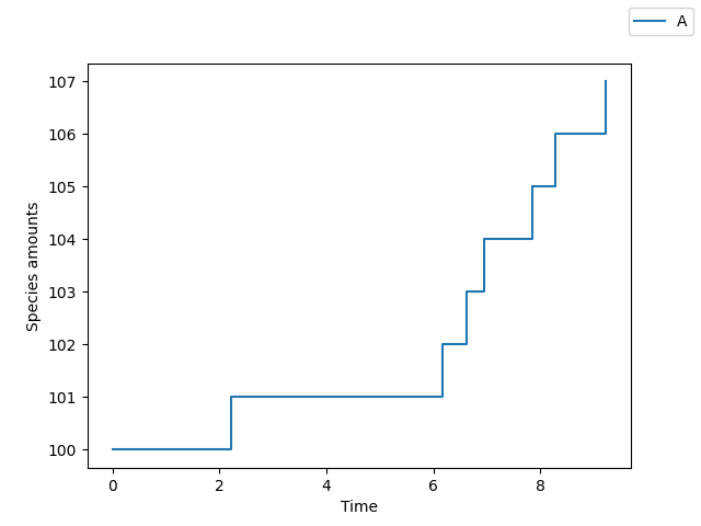
Zero order system

\[\begin{split}\phi &\xrightarrow[]{k_1} A\\ \\ k_1 &= 1.1\\ A(t=0) &= 100\\\end{split}\]

This can be coded up with:

>>> from cayenne import Simulation
>>> model_str = """
        const compartment comp1;
        comp1 = 1.0; # volume of compartment

        r1:  => A; k1;

        k1 = 1.1;
        chem_flag = false;

        A = 100;
    """
>>> sim = Simulation.load_model(model_str, "ModelString")
>>> sim.simulate()
>>> sim.plot()

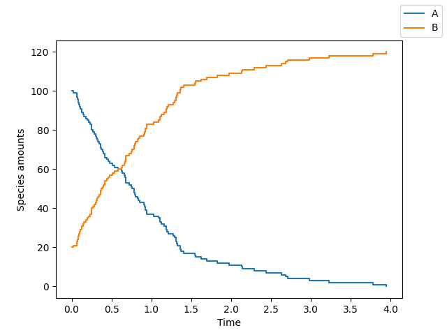
First order system

\[\begin{split}A &\xrightarrow[]{k_1} B\\ \\ k_1 &= 1.1\\ A(t=0) &= 100\\ B(t=0) &= 20\\\end{split}\]

This can be coded up with:

>>> from cayenne import Simulation
>>> model_str = """
        const compartment comp1;
        comp1 = 1.0; # volume of compartment

        r1: A => B; k1;

        k1 = 1.1;
        chem_flag = false;

        A = 100;
        B = 20;
    """
>>> sim = Simulation.load_model(model_str, "ModelString")
>>> sim.simulate()
>>> sim.plot()

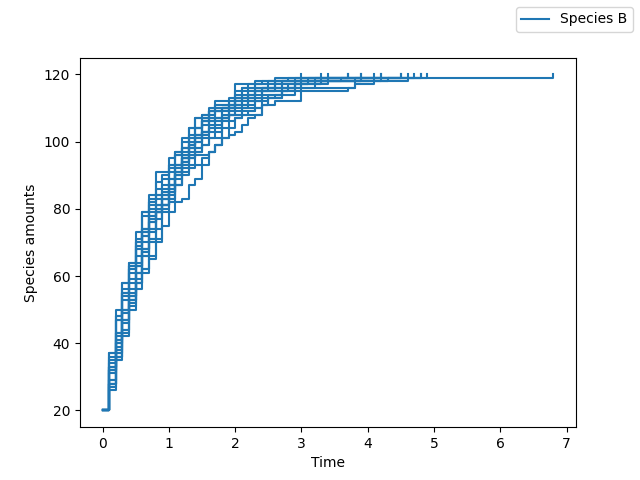
Suppose you want to use the tau_leaping algorithm, run 20 repetitions and plot only species \(B\). Then do:

>>> sim.simulate(algorithm="tau_leaping", n_rep=20)
>>> sim.plot(species_names=["B"], new_names=["Species B"])

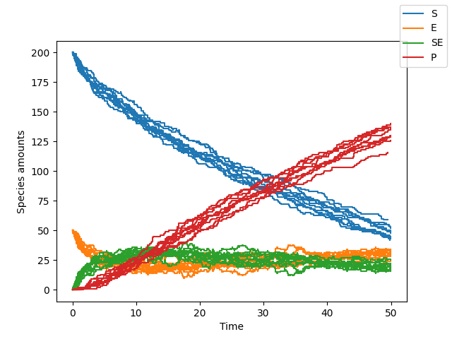
Enzyme kinetics (second order system with multiple reactions)

\[\begin{split}\text{Binding}: S + E &\xrightarrow{k1} SE \\ \text{Dissociation}:SE &\xrightarrow{k2} S + E \\ \text{Conversion}: SE &\xrightarrow{k3} P + E \\ \\ k1 &= 0.006 \\ k2 &= 0.005 \\ k3 &= 0.1 \\ S(t=0) &= 200\\ E(t=0) &= 50\\ SE(t=0) &= 0\\ P(t=0) &= 0\\\end{split}\]

This can be coded up with:

>>> from cayenne import Simulation
>>> model_str = """
        const compartment comp1;
        comp1 = 1.0; # volume of compartment

        binding: S + E => SE; k1;
        dissociation: SE => S + E; k2;
        conversion: SE => P + E; k3;

        k1 = 0.006;
        k2 = 0.005;
        k3 = 0.1;
        chem_flag = false;

        S = 200;
        E = 50;
        SE = 0;
        P = 0;
    """
>>> sim = Simulation.load_model(model_str, "ModelString")
>>> sim.simulate(max_t=50, n_rep=10)
>>> sim.plot()

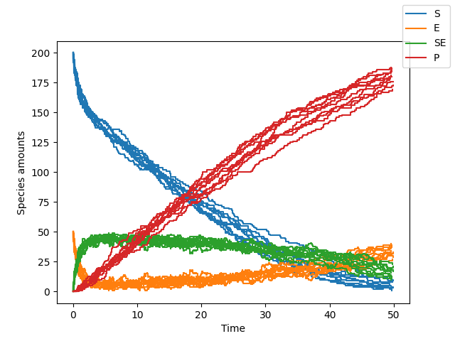
Since this is a second order system, the size of the system affects the reaction rates. What happens in a larger system?

>>> from cayenne import Simulation
>>> model_str = """
        const compartment comp1;
        comp1 = 5.0; # volume of compartment

        binding: S + E => SE; k1;
        dissociation: SE => S + E; k2;
        conversion: SE => P + E; k3;

        k1 = 0.006;
        k2 = 0.005;
        k3 = 0.1;
        chem_flag = false;

        S = 200;
        E = 50;
        SE = 0;
        P = 0;
    """
>>> sim = Simulation.load_model(model_str, "ModelString")
>>> sim.simulate(max_t=50, n_rep=10)
>>> sim.plot()

Here we see that the reaction proceeds slower. Less of the product is formed by t=50 compared to the previous case.